Chapter 6 R Markdown
R Markdown allows you to integrate formatted text (like in a Word or Google Doc), code, and code output into a single document. These documents can take many forms, including:
- html files (like this one), which allow for some interactive components, like showing/hiding code or interactive figures,
- pdf files,
- word/rich-text-format (rtf) files, for manuscripts
- and more.
The following section will guide you the process of creating an R Markdown document.
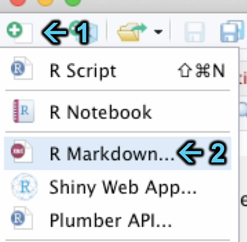
6.1 Creating an R Markdown Document
Click on the blank piece of paper with the plus sign over it in the upper left-hand corner of RStudio.
Click on
R Markdown....
- Enter the title of document and your name. I have chosen to title the document
example.

- Save your RMarkdown document by clicking on
File->Save. I’ll save thistools->scriptsfolder in myABCD 2021project.
6.2 Using an R Markdown Document
The content of R Markdown documents can be split into two main types. I will call the first type simple text. Simple text will not be evaluated by the computer other than to be formatted according to markdown syntax. If you are describing analytic decisions or interpreting the results of an analysis, you will likely be using simple text.
Note: If a comment takes up more than a line, write it in simple text, not as an R comment. Simple text can help ensure your documents are easily readable. R comments (prefaced using #) are more difficult to read and extend off the page in some Markdown formats.
Markdown syntax is used to format the simple text, such as italicizing words by enclosing them in asterisks (e.g., *this is italicized* becomes this is italicized) or bolding words by enclosing them in double-asterisks (e.g., **this is bold** becomes this is bold). For a quick rundown of what you can do with R Markdown formatting, I suggest you check out the Markdown section of the R Markdown Cheat Sheet.
In addition to simple text, R Markdown documents support R code using “chunks”. A chunk is a section of text that the document recognizes as code, rather than simple text. It will be set off in the final version of the document through different formatting. In contrast to simple text, the R code chunks are evaluated by the computer. The chunks are surrounded by ```{r} and ```. In the example image below, the 1 + 2 in the R Code chunk will be evaluated when the document is “knitted” (rendered).

6.3 Knitting an R Markdown Document
In order to knit an R Markdown document, you can either use the shortcut command + shift + k or click the button at the top of the R Markdown document that says Knit. The computer will take several seconds (or, depending on the length of the R Markdown document, several minutes) to knit the document. Once the computer has finished knitting the document, a new document will appear in the same location that the R Markdown document is saved. In this example, the new document will end with a .html extension.

As shown in the above image, the simple text in the R Markdown document on the left was rendered into a formatted in the knitted document on the right. The equation in the code chunk was also evaluated in the knitted document, returning the value 3.